E Johnson.
First published in Water e-Journal Vol 5 No 4 2020.
Abstract
Water supply and delivery inefficiencies increase the overall costs of water distribution networks, which is ultimately paid for by the customer through increased water prices or by society through cross-subsidisation. The benefits of correctly identifying and implementing efficiency improvement programs in water networks generally outweigh their costs.
The paper illustrates how the interrelationship between components of the water balance influences the derivation of water-loss performance indicators and directs the selection of loss reduction interventions. Data anomalies in one part of the balance will affect other parts due to the balance maintaining its equilibrium.
Sensitivity and scenario analysis complements the traditionally applied audit framework and overcomes previous deficiencies by determining the impact that variability of the inputs have on the variability of the outputs. The interaction between various components of the water balance was strongly influenced by supply input and customer metering errors in this example. Metered errors are valued according to customer retail unit costs, which have a higher unit value than real losses that are based on the variable production costs.
The analysis has accurately directed loss-reduction interventions that address apparent losses as well as minimise errors in the measurement of bulk supply input volumes.
Introduction
Water loss from distribution networks is a commonly adopted performance indicator by utilities for water distribution efficiency. The volumetric and financial savings can be considerable through the implementation of interventions that are aimed at reducing leakage (i.e. real) and metering (i.e. apparent) losses. Interventions that reduce operational and maintenance costs as well as increase water-use efficiencies are generally associated with lower risks and their benefits exceed the costs of their implementation. Assessing various types of water losses from a distribution network and identifying targeted interventions is facilitated by conducting water audits, which is an important approach that improves water efficiencies and avoids water wastage. When the water price that is charged to customers is designed to cover recurrent expenses, as well as funds for capital investments, inefficiencies and wastage in the distribution system will require extra funding from an increase in the cost of water. Customers will therefore ultimately be made responsible for paying for these water inefficiencies and wastage if these costs are not cross-subsidised from other income sources.
A water balance is a useful technique for assessing losses from a water distribution network through the derivation and interpretation of performance indicators. The water balance requires establishing the volumes of the various components and sub-components of the water system over a 12-month period. The standardisation of water balance structure and terminology by the International Water Association (IWA) in the late 1990s was an attempt to formalise an approach for the management and control of water losses. This approach has been adopted by national associations in various countries (e.g. including Australia, Canada, Germany, New Zealand, South Africa and USA) through the application of the IWA water balance template. Manuals detailing this water balance appoach have been developed in various countries, examples include those for Australia (Queensland EPA, 2002) and the United States (AWWA, 2016).
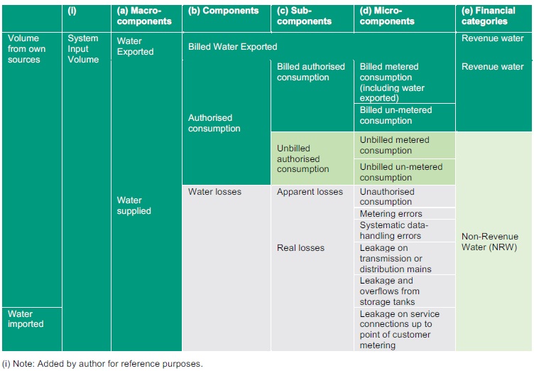
The basis of the water audit is an annual water balance that is defined by the relationship between the various components of a typical urban water system as described in Table 1.
Table 1: Urban Water Balance (AWWA, 2016)
This standardised approach facilitates the systematic review of a water utility’s records and data pertaining to the water supplied from its source and treatment, through the water distribution system, and delivered to the customers’ premises. As the quality of the data used to derive the various volumetric amounts has a direct influence on the accuracy of the resultant performance indicators, an assessment of data quality is essential. Any performance indicator is meaningless if the confidence of the input data is not known (Alegre, 2004). A water balance uncertainties approach has previously been used to illustrate the combined effect that errors in the estimates of data have on the calculation of a key water loss indicator through the determination of statistical confidence limits (Johnson, 2009). The deficiency that the water balance uncertainties approach has is that it does not determine how variability of the inputs causes variability in the outputs. A measure of the trustworthiness of data used in the water balance can also be represented by a data validation score (DVS) to rate the validity of the data as a reflection of the level of best practices employed by a water utility (AWWA, 2016). However, the use of data-grading values from one (low) to 10 (high) provides an indication of data integrity for each input value ranging from low validity (i.e. questionable data integrity) to high validity (i.e. reliable data integrity) and resultant score out of 100, but does not necessarily provide an understanding of the effects of the interaction of various anomalies.
Although the quality of data can be assessed for individual components of the water balance, the influence that data anomalies have on the resultant performance indicator because of the interaction between various components is rarely addressed in literature. This paper addresses the paucity of approaches for assessing the interrelationship between components of the water balance when deriving water-loss performance indicators. This interaction is also known as the equilibrium of the water balance that complements previous approaches by providing a mechanism for understanding the influence that these interactions have on the accuracy of various components of the balance. As such, it demonstrates the linkages between anomalies in the derivation of micro-components through to macro-components of a water balance or in any direction as dictated by the source of an anomaly and the water balance maintaining its equilibrium. It ultimately determines how variability of the inputs causes variability in the outputs.
Equilibrium of the water balance
There are a variety of water loss indicators ranging from the very simple (but biased) percentage NRW (i.e. %NRW) to the more comprehensive infrastructure leakage index (ILI) originally recommended by the IWA and endorsed by water associations in various countries. The ILI is a performance indicator quantifying how well a water system is managed for the control of real (i.e leakage) losses at the current operating pressure. Mathematically, it is the ratio of current annual real losses (CARL) to unavoidable annual real losses (UARL), or ILI=CARL/UARL. As UARL is the theoretical low limit of leakage that is technically achievable. An ILI of less than one can be because of one or combination of the following (Lambert, 2020):
- errors in low CARL volumes derived from water balances, or minimum night flows into hydraulically discrete areas and night-day factors that make allowance for the inverse relationship between water pressures and flows;
- errors in infrastructure or pressure data inputs to the UARL equation;
- lower pressure systems where the pressure and leak flow rate relationships are more sensitive than the simplified linear assumption used in the UARL equation; or
- systems where all bursts surface quickly or are easily and rapidly identified from night flow measurements, including small discrete district metered areas that facilitate leak awareness and control.
The first two points are therefore more of an indicator of data anomalies than the system’s performance, especially for water distribution networks with more than 3,000 customer connections. Water-loss indicators are established from a water balance of the water volumes entering and leaving a water system. This water balance is therefore influenced by multiple errors, including those used in the calculation of apparent losses (i.e. metering errors) and the measurement of real losses (i.e. pipeline leakage). The determination of the “top-down” water balances can be used to determine non-revenue water (NRW) and to facilitate identification of interventions required to reduce NRW. A simple but useful description of the key volumetric components identified in Table 1 is summarised in the following equations:
Water supplied = revenue water (billed volumes) + non-revenue water (unbilled volumes and losses) Equation 1
Where: non-revenue water (NRW) = apparent losses + real losses + unbilled authorised consumption Equation 2
Non-revenue water therefore represents the imbalance between the volumes of water supplied into a system and the volumes delivered to customers in the same system. Equations 1 and 2 should always be in equilibrium and, hence, any errors in the measurement of any of these components can result in the misdirection of available funds to unnecessary works or operational activities. Some common anomalies are the inaccurate measurement of water supplied by large meters or an under-estimation of customer meter errors, which result in the incorrect estimation of the volume of other components in the equilibrium equation, such as real losses and apparent losses respectively.
The management of the apparent loss component of non-revenue water must consider the various types of meter measurement errors and their interactions in the determination of water imbalances. These various error types include bias, random, weighted, combined and decay or degradation errors. Case histories have shown that without the implementation of appropriate measures to account for and report, the apparent loss volumes can be incorrectly interpreted as real loss volumes (Johnson, 2011).
Methodology
A three-stage methodology was developed to understand the influence that data anomalies can have on the accuracy of various components of the water balance due to the mechanism of its equilibrium. This is outlined as follows:
- Stage 1: Water balance calculations
A water balance is prepared as part of water loss audits and carried out according to an accepted code such as the AWWA M36 Manual (AWWA, 2016) as defined by Table 1. Steps for Stage 1 in determining the volume of non-revenue water and water losses are adapted from those by Alegre (2004), simplified to exclude the water exported row and are as follows:
Step 1. Establish macro component (column a) water supplied.
Step 2. Establish micro components (column d) billed metered consumption and billed un-metered consumption, the sum of which equals the defining category (column e), revenue water. Noting that revenue water also equates to the sub-component (column c) billed authorised consumption.
Step 3. Compute the volume of the defining category (column e) of non-revenue water by subtracting revenue water (e.g. determined in Step 2) from the water supplied (determined in Step 1).
Step 4. Establish micro components (column d) unbilled metered consumption and unbilled unmetered consumption, the sum of which equates to the sub-component (column c) unbilled authorised consumption.
Step 5. Sum the volumes of the sub-components (column c) billed authorised consumption and unbilled authorised consumption to obtain the component (column b) authorised consumption.
Step 6. Compute the component (column b) water losses by subtracting the component (column b) authorised consumption from the macro component (column a) water supplied.
Step 7. Establish micro-components (column d) unauthorised consumption and metering errors, the sum of which equates to the sub-component (column c) apparent losses.
Step 8. Compute the sub-component (column c) real losses as the component (column b) water losses (as established in Step 6) minus the sub-component (column c) apparent losses (as established in Step7).
Step 9. Validate the sub-component (column c) real losses by the best means available, which generally requires further investigations carried out after the initial audit.
The intent here is not to expand on the extensively covered topic of undertaking water audits but rather to add value to the decision-making process by using the results of these audits. The greatest benefits are in the volume and cost savings that can be achieved, by at first optimally identifying components of the water balance that are adversely impacted by interacting anomalies. The emphasis of the subsequent stages of this approach is on converting the outputs from the water audits into knowledge and intelligence to improve this decision-making process.
- Stage 2: Initial triage of audit results
The results of previous completed water loss audits are examined to determine those components of the water balance that have been assessed by the auditors as having a high priority. Initial screening of reported data and indicators is undertaken in this stage to identify those that require prioritisation for further assessment because of suspected inconsistencies, either actual or perceived. The reported results from the AWWA M36 Audits (2016) are considered further within the context of the overall assessment approach, as follows:
- Examination of previously established key volumetric and financial indicators to identify changes over several consecutive years for a specific utility as well as identify any trends between similar utilities.
- Examine the data grading value by the auditor for each input value from low to high, which is an indication of data integrity for each input value ranging from low validity (i.e. questionable data integrity) to high validity (i.e. reliable data integrity).
- Examine the three most important areas identified for investigation from the audits for the water utility.
- Determine the relative significance of the component or sub-component with respect to its volumetric (or financial) impact on the water balance (or related budget). Expressing the selected key components of the water balance as a proportion of the input supply volume (e.g. 100%). This provides a further perspective to the original auditor’s ratings and prioritisations.
- Stage 3: Sensitivity Analysis Scenarios
Sensitivity analyses for selected scenarios are developed for the water system through the interrelationship of the following three key indicators of a water balance based audit. - the infrastructure leakage index (ILI) as a derived dimensionless performance indicator for leakage;
- customer billing meter errors (%) as a derived micro-component of the water balance; and
- the measurement of the bulk water supply input (%) as a source macro-component.
Sensitivity analysis involves a process of changing the value of a particular micro-component and observing the degree this change ultimately has on the resultant value of a macro-component as well as on a key water loss performance indicator. All other input values in the water balance established from the original audit remain unaltered.
These scenarios are as follows:
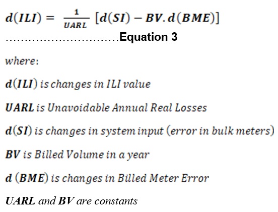
(i) Scenario 1: Bulk supply input metering errors and infrastructure leakage index. This demonstrates the linkage between anomalies in the derivation of a macro-component of a water balance (i.e. water supplied) and the derivation of a dimensionless leakage performance indicator (i.e. ILI). It also demonstrates the linkage between anomalies in a micro-component of a water balance (i.e. metering errors as % volume) and the derivation of a dimensionless leakage performance indicator (i.e. ILI). Mathematically, the relationship can be described by the following expression, with details provided in Appendix A:
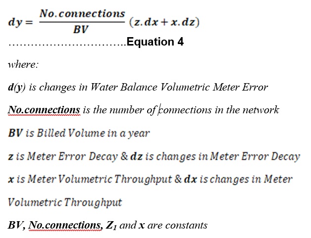
(ii) Scenario 2: Customer billing meter errors relationship with the billed volumes in the balance and the meter’s totaliser (i.e. register) reading. This demonstrates the linkage between anomalies in the derivation of a micro-component of a water balance (i.e. metering errors) and provides a validation check for this derivation process. Mathematically, the relationship can be described by the following expression, with details provided in Appendix A:
Results
Stage 2: Results of initial triage
Initial screening of the annual water audit results for four water distribution networks in California are as follows:
(i) Variations between consecutive years and utilities
The variation in water loss unit indicators between years for the same city and between cities is illustrated in Figure 1. As the accuracy of the measures are improved each year, decreases in losses between the years for the same city would be expected; however, as no water-loss reduction interventions were implemented, this is an indication of potential data anomalies. Examples are for City B’s apparent losses reduced over all the three years as well as City B, C and D’s real losses reduced between year 2 and year 3. The large increase and then decrease in real losses over the three years for cities B and C also raises suspicion as to the accuracy of the data used in the respective water audits.
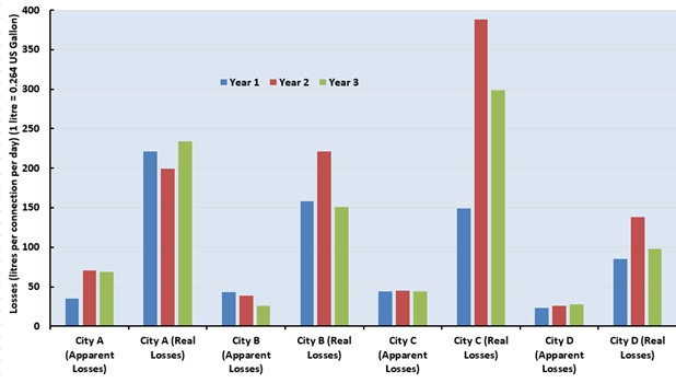 Figure 1: City and yearly comparison of apparent and real loss unit indicators
The correct extent of these losses is determined from their respective values calculated in accordance with the requirements of the AWWA M36 Manual (AWWA, 2016) and reported in the annual water loss audit as summarised for City A in Table 2. Although the volume of real losses is approximately 3.4 times greater than the volume of apparent losses, the monetary value of apparent losses is approximately 2.2 times greater than the monetary value of real losses. Reducing apparent losses by 50% will therefore have a greater value than the total cost of real losses. Implementing interventions that achieve a 50% reduction in apparent losses is feasible through the installation of digital electronic meters that are not subject to error decay and that have large operating ranges (e.g. R-ratios).
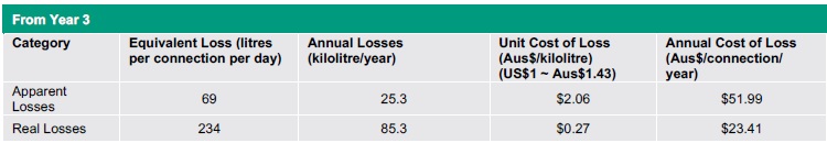 Table 2: Extent of losses for City A
(ii) Data grading value comparison
As an indication of data integrity for each input value, the auditor undertakes an assessment guided by the AWWA M36 Manual (AWWA, 2016). A summarised example is provided in Table 3. The emphasis of the existing data integrity scoring system would appear to focus on general accounting practices and is a process-based approach rather than on specific technical aspects and statistics.
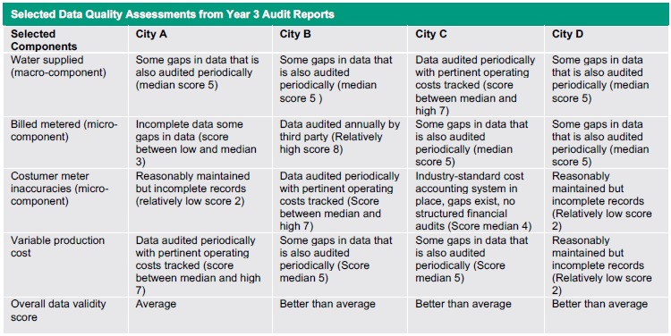 Table 3: Original auditor’s data validity ratings and scores
(iii) Previously identified most important areas
The three most important areas identified from previous water audits for each of the water utilities are listed in Table 4. The macro component, “water supplied” is the highest ranked issue for all the cities, while “micro-components of the water balance” related to customer metering dominates the second and third rankings in importance.
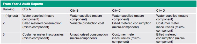 Table 4: Areas for Attention Identified by Original Auditors
(iv) Relative significance
The relative significance of the sub- and micro-components with respect to their volumetric (or financial) impact on the water balance (or related budget) provides a useful perspective as to their importance when prioritising interventions. The following key components of the water balance are expressed as a proportion of the input supply volume (i.e. 100%), which provides a further perspective to the original auditor’s ratings and prioritisations:
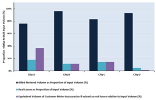 Figure 2: Relative significance of water loss components with respect to input supply volumes
- Billed metered volume as proportion of input supply volume (%).
- Real losses as proportion of input supply volume (%).
- Equivalent volume of customer meter inaccuracies as if valued as real losses (i.e. The volume of customer meter inaccuracies is multiplied by the retail unit cost of apparent losses and then divided by the variable production cost of water). This resultant “adjusted” apparent loss volume is then expressed as a proportion of the input supply volume (as %). This takes into account that metered errors have a higher unit value than real losses because they are based on customer retail unit costs (i.e. price of water to customer) while real losses are based on the variable production costs (i.e. marginal costs).
The results of this bespoke assessment are illustrated in Figure 2, which indicates that billed metered volumes account for the largest volume other than the macro-component supply input volumes which, understandably is largest for all the cities. The equivalent volume of customer meter inaccuracies is greater than that for real losses in all the cities except City D.
Stage 3: Results of sensitivity analysis
(i) Scenario 1: Bulk supply input metering under-registration
Sensitivity analysis and scenarios are developed through the interrelationship of the following three key indicators of a water balance as identified from the initial triage of audit results:
- The infrastructure leakage index (ILI).
- Customer billing meter errors (%).
- The measurement of the bulk water supply input (%) (i.e. water supplied).
Sensitivity analysis involves a process of changing the value of a particular micro-component and observing the change it ultimately has on the resultant value of a macro-component as well as changes to a key water loss performance indicator. To facilitate understanding the analysis, the permutations are initially limited to either a combination of the bulk supply meter error with that of the billing meter error or a combination of the bulk supply meter error and that of the different ILI values. The two relationships are then combined to undertake sensitivity analysis. The sensitivity of the relationship is such that increases in the bulk supply meter’s error results in an adjustment to billing meter error volumes or a different ILI value through the process of the water balance maintaining its equilibrium. This in turn, has an impact on confidence in the validity of the reported results as bulk supply meters, which are generally subjected to measurement errors. The relationship between the two values is illustrated in a chart by displaying the billing meter error field on the x-axis and the ILI on the y-axis, making it easy to see their respective relationships with that of the bulk (supply) meter error (i.e. represented by a circle/bubble graph) in Figure 3. Noting the size of the circle/bubble provides an indication as to its magnitude and only the centre of the circle relates to the values on the x- and y-axes.
Assuming that the bulk supply meter introduces an input volumetric error of 3%, for illustrative purposes, this would indicate that volumetric billing meter errors should be approximately 10.4% or with an ILI value of approximately 5.2. These values exceed the original audit values for volumetric billing meter errors of 6.4% and an ILI of 4.4. These original values do not take into account the impact that anomalies in the bulk supply input volumes have on the results even though the auditor expressed doubt regarding the validity of this data (refer to Table 3). This is indicative of how anomalies in measuring the supply input volumes can adversely affect the determination of water-loss performance indicators. As a dimensionless real loss indicator, high ILI values can be incorrectly interpreted as requiring leak reduction interventions when it could rather be the result of unaccounted for anomalies in the measurement of the input supply volumes.
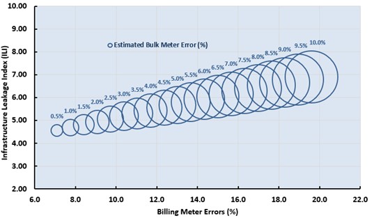 Figure 3: City A’s Sensitivity Analysis
The water audit process allows for an assessment as to the degree of error that the bulk supply meters are estimated to have, although the auditors for City A did not allow for this in the calculation of their water balance. If adjustments for these errors are not made in the volume of water supplied, it will be misrepresented and carried throughout the audit, making the quantities of apparent and real losses less certain (AWWA, 2016). Estimating these errors through the implementation of a validation process includes comparisons between the meter and a metrological reference standard. However, these validation processes require the necessary metrological accreditation, an associated quality system and one with traceability to an internationally recognised reference standard to be credible (Johnson et al., 2019). This sensitivity analysis approach for Scenario 1 is therefore useful in assessing the impact that a range of bulk meter input errors have on water-loss performance indicators to facilitate decision-making regarding proposed interventions.
(ii) Scenario 2: Customer (billing) meter errors
Although revenue (i.e. billing) meters must comply with national or international metrological standards, this compliance does not necessarily account for, nor convey, all the benefits and limitations of a particular meter or its related systems.
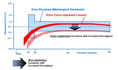 Figure 4: Meter non - and under – registration
An important aspect to consider when examining the metrology is the difference between the meter’s measurement error envelope and its error curve as illustrated in Figure 4. The error envelope relates to metrological standards and specifies the “accuracy” limits within which the meter must operate. However, the shape of the error curve within and outside this envelope is defined by the particular type of meter and has an impact on volumetric measurements, whether positive or negative.
Non-registration is the volume of water passing through the meter at flow rates lower than the starting flow rate (QStart) and is not recorded by the meter. Under-registration is the volume of water passing through the meter that is partially recorded by the meter due to mechanical wear and tear resulting from increased age or increased volumetric throughput. Deposits in some types of mechanical meters (e.g. single- and multi-jet) can result in over-registration where recorded volumes exceed the true amount passing through the meter. Some digital solid-state electronic meters can also be subject to the ad hoc occurrence of bias (systematic) measurement errors resulting in either under- or over-registration as well as the adverse influence of low scanning frequencies of the flowing water. The concept of non- and under-registration is illustrated by the movement of the error curve downward and across in Figure 4. This negative growth in meter under-registration results in meter measurement decay or degradation and establishing the condition of in-service meters together with interventions required to address these apparent losses is detailed in literature (Johnson, 2019). Non- and under-registration is water that has reached the customer but not been paid for, hence has a unit cost equivalent to the retail price of water.
The metrological quality of a meter is defined in terms of a ratio (R), which is the permanent flow rate (Q3) divided by the minimum flow rate (Q1). Installing meters with larger flow range capabilities (i.e. R-ratios) provides an intervention that minimises non-registration and minimises the adverse effects of incorrect meter sizing.
Positive displacement (i.e. oscillating piston) and nutating disc meters are especially susceptible to mechanical wear and tear, resulting in an increase in measurement errors over time and/or increased volumetric throughput. Weightings derived from “typical” customer water-usage patterns are applied to the meter measurement errors established at the various flow rates in a meter laboratory and used to derive a volumetric error that quantifies apparent losses (i.e. it converts a meter’s laboratory-determined flow rate errors to an estimated volumetric error). Hence, the volumetric error for a meter fleet is the average of all the accuracies of the meters as they operate over and beyond their respective flow range capabilities and as influenced by their in-service conditions. These in-service conditions could include those related to hydraulics (e.g. fluctuations in water pressures and flows), environmental (e.g. climatic conditions), water quality (e.g. pH, suspended solids, etc.) and asset maintenance management (e.g. in-service sampling, testing and replacement).
The water audits provide useful unit indicators for customer water-usage as well as customer meter error expressed as a percentage of billed consumption. An example for City A for Year 3 indicated an average annual usage of 360 kilolitres per customer connection per year and a customer meter volumetric error of -6.4% of the billed volume. Sensitivity analysis involving assessing their meter decay rates and their volumetric throughputs provide a means to assess the validity of the previous audit results.
The expected range of error decay (i.e. under-registration) for mechanical meters measuring customer usage varies between -0.1% and -0.6% per year (Noss et al., 1987). The overall volumetric error of the billing meters (y-axis) is derived from the meter’s volumetric throughput (x-axis) and the meter’s error decay per year (the linear graphs) as illustrated in the example in Figure 5. City A’s example of the audit determined -6.4% customer meter volumetric error, if the total volumetric throughput per meter (i.e. from meter’s totaliser/register readings) was 3,900 kilolitres then the meter error decay would be on average -0.6% per annum. The average age for City A’s meter fleet would therefore be approximately 10.8 years (i.e. 3,900 kL divided by 360 kL/conn./yr). A note of caution is that a low average meter age or volumetric throughput could also be incorrectly interpreted as the fleet could consist of relatively new mechanical meters or consist of electronic digital meters that are not generally subjected to measurement error decay. Reiterating that reference to Figure 4 relates to meter measurement error with respect to a particular flow rate through the meter and Figure 5 relates to the meter’s volumetric error with respect to the characteristic water usage pattern (i.e. demand profile) monitored by the meter. Confusion between these two concepts can result in the incorrect selection of default values for billing meters in the water balance–based audit.
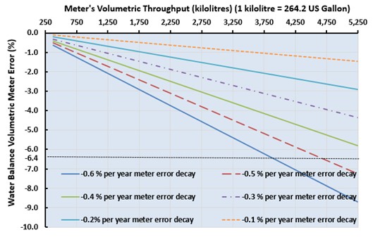 Figure 5: Example of Volumetric and Meter Error Decay Relationship for City A
Various combinations are applied to determine the veracity of the reported customer meter volumetric errors as compared to the customer meters’ error decay with the average total volumetric throughput of the meter fleet, the average age of the meter fleet and the average annual water usage per meter (from billing and asset records). In the case when meter error decay has not been determined from sampling and testing in-service meters, it can be approximated by changing the error decay rate until it matches the billing records of average total volumetric throughput for the whole fleet and the water balance derived volumetric meter error. The accuracy of the derived decay rates can ultimately only be established from the sampling and testing of in-service meters; however, unless there is a good reason to believe otherwise, decay rates outside the range of -0.1% to -0.6% per year provide a strong indication that there are anomalies in the water balance derived values. Noting again that these decay rates are referring to weighted volumetric errors derived from meter error curves and water usage patterns.
Discussion
Inefficiencies and wastage of water increases the overall costs of water distribution networks, which is ultimately paid for by the customer through inceased water prices or by society through cross-subsidisation. Identifying and quantifying these inefficiencies require the preparation of a volumetric balance of the water flowing into and out of the network for a given period. The quality of various data has a direct influence on the accuracy of the resultant efficiency indicators. Although there are several examples in literature dealing with establishing the confidence of the data as well as the combined effect that errors have on the results of a water balance, there is scarcity of references that demonstrates the sensitivity of derived indicators to the variability of the original data.
This paper attempts to address the paucity of approaches for assessing the interrelationship between components of the water balance when deriving water efficiency indicators. This interaction is also known as the equilibrium of the water balance and provides a mechanism for understanding the influence that these interrelationships have on the accuracy of various components of the balance. As such, it demonstrates the linkages between anomalies in the derivation of micro-components through to macro-components of a water balance or in any direction as dictated by the source of an anomaly and the water balance maintaining its equilibrium. It complements previous approaches by quantifying the effects that uncertainties in the water balance’s input data have on the resultant efficiency indicators.
Data anomalies mask the results of water-loss audits based on an internationally adopted water balance approach. The negative impact that these anomalies have on decision-making can be minimised through the creation of useful information through the application of an improved approach.
The outcomes of the analysis reflect that metered errors have a higher unit value than real losses, as they are based on customer retail unit costs (i.e. price of water to the customer) while real losses are based on variable production costs (i.e. marginal costs). Anomalies in measuring the supply input volumes can also adversely affect the determination of water loss performance indicators. As a dimensionless real loss indicator, high ILI values can be incorrectly interpreted as requiring leak reduction interventions when they are in fact the result of unaccounted for anomalies in the measurement of the input supply volumes or customer billing meter errors.
Sensitivity and scenario analysis complements the traditionally applied audit framework and overcomes the deficiencies of previous assessment processes by determining the impact that variability of the volumetric inputs have on the variability of the resultant indicators. It provides a unique perspective of the interaction between various components of the water balance, which in this example was strongly influenced by supply input and customer metering errors.The sensitivity analysis approach undertaken for the following scenarios demontrated that for:
- Scenario 1: The impact that a range of bulk meters’ input errors have on water loss performance indicators. This facilitates decision making regarding the correct identification of the part of the water balance requiring emphasis through focussed interventions.
- Scenario 2: The impact that customer billing meter errors have on the billed volumes, which also provides an indication of the meter’s in-service performance. Potential anomalies can also be further assessed in terms of the asset’s performance characteristics under these operational in-service conditions.
The analysis has accurately directed loss reduction interventions that address apparent losses as well as minimise errors in the measurement of bulk supply input volumes.
Conclusions
The three-stage approach progressively refines the outputs from the traditional water audit process that produces information to enhance decision-making. This restricts the adverse impact that anomalies in the original data have on incorrectly identifying water loss reduction interventions. It also emphasises the value of the various categories of losses rather than solely their volumes. Sensitivity and scenario analysis complement the traditionally applied audit framework, fills the gap in interpreting the results and reinforces the findings of annual water audits. This provides a unique perspective of the interaction between various components of the water balance, which in this example was strongly influenced by supply input and customer metering errors. This approach has accurately directed the following water loss reduction programs:
- Minimise errors in the measurement of bulk supply input volumes through the implementation of a validation process that makes a comparison of the meter with that of a metrological reference standard, includes the necessary metrological accreditation and associated quality system and traceability to an internationally recognised reference standard (Johnson et al., 2019).
- Reduce apparent losses through a comprehensive condition assessment of in-service meters that informs those interventions that include development of meter replacement programs, replacement with meters that are not subject to error decay and selection of meters with large operating ranges (Johnson, 2019).
Acknowledgements
The following are gratefully acknowledged for their assistance:
- Solano County Water Agency, California, USA, for permission to use the data in this paper.
- Professor JE (Kobus) van Zyl Ph.D., Watercare Chair in Infrastructure, Department of Civil and Environmental Engineering, University of Auckland for his review of this paper.
- Associate Professor in Statistics, Dr Andrew Metcalfe, School of Mathematical Sciences, the University of Adelaide for his review of the mathematical expressions and derivations detailed in this paper.
- Comments provided by Keith Roberts and Richard Savage (from GHD).
- Assistance with the analysis by Sareh Darreh (from GHD).
About the author
Edgar Johnson | Edgar is a professional engineer with more than 35 years of Australian and International experience in water management. His education combines a Doctor of Technology with a commerce degree, providing him with unique insight into the full range of utility system practices. He has developed standards and guidelines associated with water loss management, efficiency and metering and has published more than 30 related articles/papers/research books. His involvement with the International Water Association (IWA) Water Loss Specialist Group included leadership of its non-revenue water apparent loss (AL) initiative. He was selected as one of 30 of Australia's Most Innovative Engineers by Engineers Australia in 2017. He is currently a Senior Technical Director: Water Efficiency at GHD.
Appendix
References
Alegre, H.(2006). Performance Indicators as a Management Support Tool. Published in Urban Water Supply Management Tools. Editor-in-Chief, Mays ,L.W. Published by McGraw-Hill. ISBN 0-07-142836-4
American Water Works Association (2016). Water Audits and Loss Control Programs. Manual M36. Fouth Edition. Managing Editor Valentine, M. ISBN-13 978-1-62576-100-2
Johnson, E.H. (2009). Management of Non-revenue and Revenue Water Data. Engineers Media, Australia. ISBN 9780858258839 (2nd Edition).
Johnson, E.H. (2011). The ‘Apparent’ Real Losses of a Water Balance. IWA Efficient 2011 Conference. March. Jordan.
Johnson, E.H. (2019). Enhancing Water Meter In-service Testing and Replacement Decisions. AWA Water eJournal. Vol. 4 No.1
Johnson, E.H., Mueller, U. & Savage, R. (2019). Innovative Laser Doppler Velocimetry (LDV) Technique Improves the In-field Accuracy Assessments of Large Water Meters. American Water Works Association (AWWA) ACE’19 Conference, Denver Co. USA
Lambert, A (2020). Low ILIs and Small Systems -System Correction Factor SCF can customise the standard UARL equation for pipe materials, small systems and pressure: bursts relationships. acccessed 14 September 2020. Leakssuite Library Ltd. https://www.leakssuitelibrary.com/low-ilis-and-small-systems
Noss R.R., Newman G.J. & Male J.W. (1987). Optimal Testing Frequency for Domestic Water Meters. Journal of Water Resources Planning and Management Vol 113, No. 1 January.
Queensland Environmental Protection Agency (2002). Managing and Reducing Water Losses from Water Distribution Systems. Manual 2: Water Audits. ISBN 0724294929
Share